[팀 프로젝트] AI가 쓴 글과 인간이 쓴 글 분류하는 인공지능 만들기 프로젝트

사용한 데이터: https://aihub.or.kr/aihubdata/data/view.do?pageIndex=2&currMenu=115&topMenu=100&srchOptnCnd=OPTNCND001&searchKeyword=%EC%9A%94%EC%95%BD%EB%AC%B8&srchDetailCnd=DETAILCND001&srchOrder=ORDER001&srchPagePer=20&aihubDataSe=data&dataSetSn=582 / 해당 데이터 기반으로 AI가 생성한 AI 텍스트 데이터 (동일 글 서식, 주제로 작성)

1. 기존 모델

1-1. 기존 모델 코드

모델 코드

import pandas as pd
import numpy as np
import pickle
import re
from sklearn.linear_model import LogisticRegression
from sklearn.model_selection import train_test_split, cross_val_score
from sklearn.metrics import classification_report, accuracy_score
from sklearn.preprocessing import StandardScaler

# ─────────────────────────────────────────
# 1. 데이터 로드
# ─────────────────────────────────────────
data = pd.read_csv('labeled_dataset.csv').dropna(subset=['text'])
print(f"총 데이터: {len(data)}건 (human: {(data['label']==0).sum()}, AI: {(data['label']==1).sum()})")

# ─────────────────────────────────────────
# 2. 언어적 특징 추출 함수 (text_len 제외)
# ─────────────────────────────────────────
AI_CONJUNCTIONS = ['또한', '따라서', '그러나', '하지만', '이에', '이를', '이로', '한편', '더불어', '아울러']

def extract_features(text: str) -> dict:
    if not isinstance(text, str) or len(text) == 0:
        return {k: 0 for k in ['avg_sent_len', 'std_sent_len', 'vocab_diversity',
                                'conjunction_ratio', 'comma_ratio', 'period_count', 'avg_word_len']}
    sentences = [s.strip() for s in re.split(r'[.!?]', text) if s.strip()]
    sent_lens = [len(s) for s in sentences] if sentences else [0]
    words = text.split()
    unique_words = set(words)
    conjunction_count = sum(text.count(c) for c in AI_CONJUNCTIONS)
    return {
        'avg_sent_len':      np.mean(sent_lens),
        'std_sent_len':      np.std(sent_lens),
        'vocab_diversity':   len(unique_words) / len(words) if words else 0,
        'conjunction_ratio': conjunction_count / len(words) if words else 0,
        'comma_ratio':       text.count(',') / len(text),
        'period_count':      text.count('.') / len(text),
        'avg_word_len':      np.mean([len(w) for w in words]) if words else 0,
    }

print("특징 추출 중...")
X = pd.DataFrame([extract_features(t) for t in data['text']])
y = data['label']
print(f"특징 벡터 shape: {X.shape}")

# ─────────────────────────────────────────
# 3. 모델 학습
# ─────────────────────────────────────────
scaler = StandardScaler()
X_scaled = scaler.fit_transform(X)

X_train, X_test, y_train, y_test = train_test_split(
    X_scaled, y, test_size=0.2, random_state=42, stratify=y
)

model = LogisticRegression(max_iter=1000, random_state=42, solver='lbfgs')
model.fit(X_train, y_train)

# ─────────────────────────────────────────
# 4. 성능 평가
# ─────────────────────────────────────────
y_pred = model.predict(X_test)
print("\n=== 전체 성능 ===")
print(f"Accuracy: {accuracy_score(y_test, y_pred)*100:.1f}%")
print(classification_report(y_test, y_pred, target_names=['Human', 'AI']))

print("=== 도메인별 정확도 ===")
data_copy = data.copy()
data_copy['pred_label'] = model.predict(scaler.transform(
    pd.DataFrame([extract_features(t) for t in data_copy['text']])
))
for domain in data['domain'].unique():
    subset = data_copy[data_copy['domain'] == domain]
    acc = accuracy_score(subset['label'], subset['pred_label'])
    print(f"  {domain}: {acc*100:.1f}%")

cv_scores = cross_val_score(model, X_scaled, y, cv=5)
print(f"\n5-fold CV 평균: {cv_scores.mean()*100:.1f}% (±{cv_scores.std()*100:.1f}%)")

feat_importance = pd.Series(np.abs(model.coef_[0]), index=X.columns).sort_values(ascending=False)
print("\n=== 특징 중요도 ===")
print(feat_importance)

# ─────────────────────────────────────────
# 5. 모델 저장
# ─────────────────────────────────────────
with open('ai_detector_model.pkl', 'wb') as f:
    pickle.dump({'model': model, 'scaler': scaler}, f)
print("\n모델 저장 완료: ai_detector_model.pkl")

# ─────────────────────────────────────────
# 6. 실제 사용 함수
# ─────────────────────────────────────────
def detect_ai(text: str) -> float:
    features = pd.DataFrame([extract_features(text)])
    features_scaled = scaler.transform(features)
    prob = model.predict_proba(features_scaled)[0][1]
    print(f"\n입력 텍스트: {text[:50]}...")
    print(f"→ AI가 썼을 확률: {prob*100:.1f}%")
    return prob

print("\n=== 실제 감지 테스트 ===")
sample_human = data[data['label']==0]['text'].iloc[0]
sample_ai    = data[data['label']==1]['text'].iloc[0]
detect_ai(sample_human)
detect_ai(sample_ai)

결과

총 데이터: 2400건 (human: 1200, AI: 1200)
특징 추출 중...
특징 벡터 shape: (2400, 7)

=== 전체 성능 ===
Accuracy: 85.4%
              precision    recall  f1-score   support

       Human       0.87      0.83      0.85       240
          AI       0.84      0.88      0.86       240

    accuracy                           0.85       480
   macro avg       0.85      0.85      0.85       480
weighted avg       0.85      0.85      0.85       480

=== 도메인별 정확도 ===
  news: 81.3%
  edit: 85.2%
  speech: 84.5%
  literature: 87.2%

5-fold CV 평균: 78.3% (±4.8%)

=== 특징 중요도 ===
std_sent_len         4.288583
avg_sent_len         1.515089
avg_word_len         0.540784
comma_ratio          0.513366
vocab_diversity      0.465062
conjunction_ratio    0.360234
period_count         0.227850
dtype: float64

모델 저장 완료: ai_detector_model.pkl

=== 실제 감지 테스트 ===

입력 텍스트: 집단감염이 발생한 서울 구로구 보험사 콜센터와 관련한 신종 코로나바이러스 감염증(코로나19...
→ AI가 썼을 확률: 0.9%

입력 텍스트: 서울 구로구 신도림동 코리아빌딩에 입주한 한 보험사 콜센터에서 발생한 코로나19 집단감염 ...
→ AI가 썼을 확률: 79.0%

2. 실제 테스트 코드 및 결과

1. 실제 테스트 코드

실제 테스트 코드

import pickle
import pandas as pd
import numpy as np
import re
import matplotlib.pyplot as plt


# ── 모델 로드 ──────────────────────────────────────
with open('ai_detector_model.pkl', 'rb') as f:
    saved = pickle.load(f)
model  = saved['model']
scaler = saved['scaler']

AI_CONJUNCTIONS = ['또한', '따라서', '그러나', '하지만', '이에', '이를', '이로', '한편', '더불어', '아울러']
FEAT_KO = ['평균 문장 길이', '문장 길이 편차', '어휘 다양성',
           '접속어 비율', '쉼표 밀도', '마침표 밀도', '평균 단어 길이']

def extract_features(text):
    if not isinstance(text, str) or len(text) == 0:
        return {k: 0 for k in ['avg_sent_len', 'std_sent_len', 'vocab_diversity',
                                'conjunction_ratio', 'comma_ratio', 'period_count', 'avg_word_len']}
    sentences = [s.strip() for s in re.split(r'[.!?]', text) if s.strip()]
    sent_lens = [len(s) for s in sentences] if sentences else [0]
    words = text.split()
    unique_words = set(words)
    conjunction_count = sum(text.count(c) for c in AI_CONJUNCTIONS)
    return {
        'avg_sent_len':      np.mean(sent_lens),
        'std_sent_len':      np.std(sent_lens),
        'vocab_diversity':   len(unique_words) / len(words) if words else 0,
        'conjunction_ratio': conjunction_count / len(words) if words else 0,
        'comma_ratio':       text.count(',') / len(text),
        'period_count':      text.count('.') / len(text),
        'avg_word_len':      np.mean([len(w) for w in words]) if words else 0,
    }

def explain(text):
    feat = extract_features(text)
    feat_df = pd.DataFrame([feat])
    feat_scaled = scaler.transform(feat_df)
    prob = model.predict_proba(feat_scaled)[0][1]
    contributions = feat_scaled[0] * model.coef_[0]

    print(f"\n{'='*50}")
    print(f"입력 텍스트: {text[:60]}{'...' if len(text)>60 else ''}")
    print(f"AI가 썼을 확률: {prob*100:.1f}%")
    print(f"{'='*50}")
    print(f"{'특징':<18} {'값':>10}  {'기여도':>8}  방향")
    print('-'*50)
    for ko, val, contrib in zip(FEAT_KO, feat_df.values[0], contributions):
        direction = "→ AI" if contrib > 0 else "→ 사람"
        print(f"{ko:<16} {val:>10.4f}  {contrib:>+8.3f}  {direction}")
    print(f"{'='*50}\n")

    fig, axes = plt.subplots(1, 2, figsize=(13, 5))
    fig.suptitle(f'추론 과정  |  AI 확률: {prob*100:.1f}%', fontsize=14, fontweight='bold')

    ax1 = axes[0]
    colors = ['#D4537E' if c > 0 else '#378ADD' for c in contributions]
    bars = ax1.barh(FEAT_KO, contributions, color=colors, height=0.6)
    ax1.axvline(0, color='gray', linewidth=0.8, linestyle='--')
    ax1.set_xlabel('기여도 (양수=AI, 음수=사람)')
    ax1.set_title('특징별 기여도')
    for bar, val in zip(bars, contributions):
        ax1.text(val + (0.01 if val >= 0 else -0.01), bar.get_y() + bar.get_height()/2,
                 f'{val:+.3f}', va='center', ha='left' if val >= 0 else 'right', fontsize=9)

    ax2 = axes[1]
    norm_vals = feat_scaled[0]
    colors2 = ['#D4537E' if v > 0 else '#378ADD' for v in norm_vals]
    ax2.barh(FEAT_KO, norm_vals, color=colors2, height=0.6, alpha=0.7)
    ax2.axvline(0, color='gray', linewidth=0.8, linestyle='--')
    ax2.set_xlabel('표준화된 특징값 (0 = 평균)')
    ax2.set_title('특징값 (평균 대비)')

    from matplotlib.patches import Patch
    legend = [Patch(color='#D4537E', label='AI 쪽'), Patch(color='#378ADD', label='사람 쪽')]
    ax1.legend(handles=legend, loc='lower right', fontsize=9)

    plt.tight_layout()
    plt.savefig('explain_result.png', dpi=150, bbox_inches='tight')
    plt.show()
    print("explain_result.png 저장됨")

my_text = """
"""

ai_text = """

"""

explain(my_text)
explain(ai_text)

2. 결과

1. 사람이 쓴 글

2. AI가 쓴 글

2-3. 기존 방식 정리

기존 모델은 수동 특징 추출 기반의 Logistic Regression. 텍스트에서 7가지 언어적 특징을 직접 손으로 계산해서 분류기에 넣는 방식이었다.

문제점

수작업으로 만든 특징들은 AI 글쓰기의 패턴을 너무 단순하게 요약할 수 있다. 예를 들어 접속어 비율이나 문장 길이 같은 거시적 통계는 AI와 사람의 실제 언어 패턴 차이를 충분히 잡아내지 못한다. 또한 이 특징들은 도메인이나 글 길이에 따라 값이 크게 달라지기 때문에 일반화 성능이 낮을 수밖에 없었다.

2. Logistic Regression (개선안)

2-1. 모델 코드

모델 코드

import pickle
import pandas as pd

from sklearn.model_selection import train_test_split, cross_val_score, StratifiedKFold
from sklearn.pipeline import Pipeline, FeatureUnion
from sklearn.feature_extraction.text import TfidfVectorizer
from sklearn.linear_model import LogisticRegression
from sklearn.metrics import accuracy_score, classification_report, confusion_matrix, f1_score


# ─────────────────────────────────────────
# 1. 데이터 로드
# ─────────────────────────────────────────
data = pd.read_csv("labeled_dataset.csv").dropna(subset=["text", "label"]).copy()
data["text"] = data["text"].astype(str)
data["label"] = data["label"].astype(int)

print(f"총 데이터: {len(data)}건")
print(f"Human: {(data['label'] == 0).sum()}건")
print(f"AI: {(data['label'] == 1).sum()}건")


# ─────────────────────────────────────────
# 2. 학습 / 테스트 분리
# ─────────────────────────────────────────
X_train, X_test, y_train, y_test = train_test_split(
    data["text"],
    data["label"],
    test_size=0.2,
    random_state=42,
    stratify=data["label"]
)


# ─────────────────────────────────────────
# 3. Feature 구성
# ─────────────────────────────────────────
features = FeatureUnion([
    ("char_tfidf", TfidfVectorizer(
        analyzer="char",
        ngram_range=(3, 5),
        min_df=2,
        max_features=50000,
        sublinear_tf=True,
        lowercase=False
    )),
    ("word_tfidf", TfidfVectorizer(
        analyzer="word",
        ngram_range=(1, 2),
        min_df=2,
        max_features=30000,
        sublinear_tf=True,
        lowercase=False
    ))
])


# ─────────────────────────────────────────
# 4. 모델 구성
# ─────────────────────────────────────────
model = Pipeline([
    ("features", features),
    ("clf", LogisticRegression(
        solver="saga",
        max_iter=3000,
        C=2.0,
        class_weight="balanced",
        n_jobs=-1,
        random_state=42
    ))
])


# ─────────────────────────────────────────
# 5. 학습
# ─────────────────────────────────────────
print("\n[Logistic Regression 학습 시작]")
model.fit(X_train, y_train)


# ─────────────────────────────────────────
# 6. 테스트 평가
# ─────────────────────────────────────────
y_pred = model.predict(X_test)

print("\n=== Logistic Regression Test 성능 ===")
print(f"Accuracy: {accuracy_score(y_test, y_pred) * 100:.2f}%")
print(f"F1 macro: {f1_score(y_test, y_pred, average='macro'):.4f}")
print(classification_report(y_test, y_pred, target_names=["Human", "AI"], zero_division=0))
print("Confusion matrix:")
print(confusion_matrix(y_test, y_pred))


# ─────────────────────────────────────────
# 7. 교차검증
# ─────────────────────────────────────────
cv = StratifiedKFold(n_splits=3, shuffle=True, random_state=42)

cv_scores = cross_val_score(
    model,
    data["text"],
    data["label"],
    cv=cv,
    scoring="f1_macro",
    n_jobs=-1
)

print("\n=== 3-fold CV ===")
print(f"f1_macro: {cv_scores.mean():.4f} (± {cv_scores.std():.4f})")


# ─────────────────────────────────────────
# 8. 저장
# ─────────────────────────────────────────
with open("ai_detector_lr.pkl", "wb") as f:
    pickle.dump(model, f)

print("\n모델 저장 완료: ai_detector_lr.pkl")

결과

총 데이터: 2400건
Human: 1200건
AI: 1200건

[Logistic Regression 학습 시작]

=== Logistic Regression Test 성능 ===
Accuracy: 99.79%
F1 macro: 0.9979
              precision    recall  f1-score   support

       Human       1.00      1.00      1.00       240
          AI       1.00      1.00      1.00       240

    accuracy                           1.00       480
   macro avg       1.00      1.00      1.00       480
weighted avg       1.00      1.00      1.00       480

Confusion matrix:
[[239   1]
 [  0 240]]

=== 3-fold CV ===
f1_macro: 0.9921 (± 0.0006)

모델 저장 완료: ai_detector_lr.pkl

2-2. 실제 테스트 코드 및 결과

1. 실제 테스트 코드

테스트 코드

import pickle
import numpy as np
import matplotlib.pyplot as plt

# 한글 깨지면 사용
# import koreanize_matplotlib


# ─────────────────────────────────────────
# 모델 로드
# ─────────────────────────────────────────
with open("ai_detector_model.pkl", "rb") as f:
    model = pickle.load(f)


# 개선 모델 구조:
# model = Pipeline([
#     ("features", FeatureUnion([...]))
#     ("clf", LogisticRegression(...))
# ])

features = model.named_steps["features"]
clf = model.named_steps["clf"]


# ─────────────────────────────────────────
# FeatureUnion의 feature 이름 가져오기
# ─────────────────────────────────────────
def get_feature_names_from_union(feature_union):
    feature_names = []

    for name, transformer in feature_union.transformer_list:
        names = transformer.get_feature_names_out()

        # char_tfidf__문자패턴, word_tfidf__단어패턴 형태로 표시
        names = [f"{name}__{feature}" for feature in names]
        feature_names.extend(names)

    return np.array(feature_names)


feature_names = get_feature_names_from_union(features)


# ─────────────────────────────────────────
# 설명 함수
# ─────────────────────────────────────────
def explain(text, top_n=15):
    # 벡터화
    X = features.transform([text])

    # 예측
    prob = model.predict_proba([text])[0][1]
    pred = model.predict([text])[0]

    # 현재 문서에서 실제로 등장한 feature들
    indices = X.indices
    values = X.data

    # 각 feature의 기여도 계산
    coef = clf.coef_[0]
    contributions = values * coef[indices]

    # 기여도 절댓값 기준 상위 feature 추출
    order = np.argsort(np.abs(contributions))[::-1][:top_n]

    top_features = feature_names[indices][order]
    top_contribs = contributions[order]
    top_values = values[order]

    # ─────────────────────────────────────
    # 출력
    # ─────────────────────────────────────
    print(f"\n{'=' * 70}")
    print(f"입력 텍스트: {text[:80]}{'...' if len(text) > 80 else ''}")
    print(f"예측 라벨: {'AI' if pred == 1 else 'Human'}")
    print(f"AI 확률: {prob * 100:.2f}%")
    print(f"{'=' * 70}")

    print(f"\n{'특징':<35} {'TF-IDF':>10} {'기여도':>12} 방향")
    print("-" * 70)

    for feat, val, contrib in zip(top_features, top_values, top_contribs):
        direction = "→ AI" if contrib > 0 else "→ 사람"
        print(f"{feat:<35} {val:>10.4f} {contrib:>+12.4f} {direction}")

    # ─────────────────────────────────────
    # 시각화
    # ─────────────────────────────────────
    fig, axes = plt.subplots(1, 2, figsize=(16, 6))

    fig.suptitle(
        f"AI 판별 분석 | AI 확률: {prob * 100:.1f}%",
        fontsize=15,
        fontweight="bold"
    )

    # 1. feature contribution
    ax1 = axes[0]

    colors = ["#D4537E" if c > 0 else "#378ADD" for c in top_contribs]

    bars = ax1.barh(
        range(len(top_features)),
        top_contribs,
        color=colors,
        height=0.7
    )

    ax1.set_yticks(range(len(top_features)))
    ax1.set_yticklabels(top_features)
    ax1.axvline(0, color="gray", linestyle="--")
    ax1.set_title("특징별 기여도")
    ax1.set_xlabel("양수 = AI / 음수 = 사람")

    for bar, val in zip(bars, top_contribs):
        ax1.text(
            val + (0.001 if val >= 0 else -0.001),
            bar.get_y() + bar.get_height() / 2,
            f"{val:+.3f}",
            va="center",
            ha="left" if val >= 0 else "right",
            fontsize=8
        )

    # 2. TF-IDF 값
    ax2 = axes[1]

    bars2 = ax2.barh(
        range(len(top_features)),
        top_values,
        color=colors,
        alpha=0.75,
        height=0.7
    )

    ax2.set_yticks(range(len(top_features)))
    ax2.set_yticklabels(top_features)
    ax2.set_title("TF-IDF 값")
    ax2.set_xlabel("등장 강도")

    for bar, val in zip(bars2, top_values):
        ax2.text(
            val + 0.001,
            bar.get_y() + bar.get_height() / 2,
            f"{val:.3f}",
            va="center",
            fontsize=8
        )

    plt.tight_layout()
    plt.savefig("explain_result.png", dpi=150, bbox_inches="tight")
    plt.show()

    print("\nexplain_result.png 저장 완료")
    print(f"{'=' * 70}\n")
my_text = """
"""

ai_text = """

"""

explain(my_text)
explain(ai_text)

2. 테스트 결과

1) 사람이 쓴 글

2) AI가 쓴 글

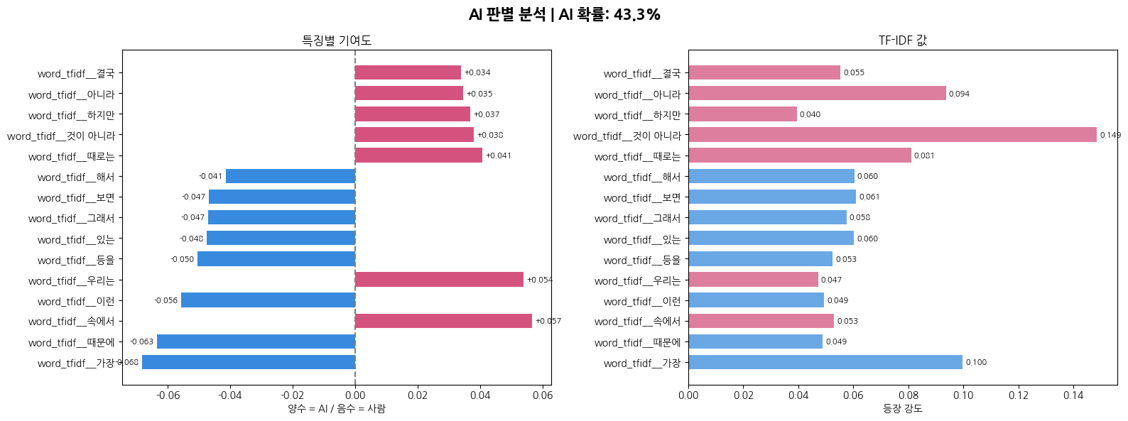
2-3. 기존과의 차이점

수동 특징 대신 TF-IDF 벡터화로 특징을 자동 추출. 두 종류의 TF-IDF를 FeatureUnion으로 결합함.

• char n-gram TF-IDF: AI 글에서 자주 반복되는 자음/음절 패턴을 포착. 마치 지문처럼 AI 특유의 글자 조합 습관을 잡아냄.
• word n-gram TF-IDF: AI가 반복적으로 사용하는 어구나 단어 조합을 포착.

2-4. 이 모델을 사용한 이유

기존의 손수 만든 특징 7개로는 놓치는 패턴이 많지만 TF-IDF는 수만 개의 텍스트 패턴을 자동으로 학습해서 훨씬 풍부하게 표현이 가능함. Logistic Regression 은 계수를 통해 어떤 패턴이 AI/사람 방향으로 기여했는지 해석이 가능함. 따라서 설명 가능성 측면에서 유리함.

3. LinearSVC+TF-IDF

3-1. 모델 코드 및 결과

모델 코드

import pickle
import pandas as pd

from sklearn.model_selection import train_test_split, cross_val_score, StratifiedKFold
from sklearn.pipeline import Pipeline, FeatureUnion
from sklearn.feature_extraction.text import TfidfVectorizer
from sklearn.svm import LinearSVC
from sklearn.calibration import CalibratedClassifierCV
from sklearn.metrics import accuracy_score, classification_report, confusion_matrix, f1_score


# ─────────────────────────────────────────
# 1. 데이터 로드
# ─────────────────────────────────────────
data = pd.read_csv("labeled_dataset.csv").dropna(subset=["text", "label"]).copy()
data["text"] = data["text"].astype(str)
data["label"] = data["label"].astype(int)

print(f"총 데이터: {len(data)}건")
print(f"Human: {(data['label'] == 0).sum()}건")
print(f"AI: {(data['label'] == 1).sum()}건")


# ─────────────────────────────────────────
# 2. 학습 / 테스트 분리
# ─────────────────────────────────────────
X_train, X_test, y_train, y_test = train_test_split(
    data["text"],
    data["label"],
    test_size=0.2,
    random_state=42,
    stratify=data["label"]
)


# ─────────────────────────────────────────
# 3. Feature 구성
# ─────────────────────────────────────────
features = FeatureUnion([
    ("char_tfidf", TfidfVectorizer(
        analyzer="char",
        ngram_range=(3, 5),
        min_df=2,
        max_features=50000,
        sublinear_tf=True,
        lowercase=False
    )),
    ("word_tfidf", TfidfVectorizer(
        analyzer="word",
        ngram_range=(1, 2),
        min_df=2,
        max_features=30000,
        sublinear_tf=True,
        lowercase=False
    ))
])


# ─────────────────────────────────────────
# 4. 모델 구성
# ─────────────────────────────────────────
base_svc = LinearSVC(
    C=1.0,
    class_weight="balanced",
    random_state=42,
    max_iter=5000
)

svc_with_prob = CalibratedClassifierCV(
    base_svc,
    cv=3
)

model = Pipeline([
    ("features", features),
    ("clf", svc_with_prob)
])


# ─────────────────────────────────────────
# 5. 학습
# ─────────────────────────────────────────
print("\n[LinearSVC 학습 시작]")
model.fit(X_train, y_train)


# ─────────────────────────────────────────
# 6. 테스트 평가
# ─────────────────────────────────────────
y_pred = model.predict(X_test)

print("\n=== LinearSVC Test 성능 ===")
print(f"Accuracy: {accuracy_score(y_test, y_pred) * 100:.2f}%")
print(f"F1 macro: {f1_score(y_test, y_pred, average='macro'):.4f}")
print(classification_report(y_test, y_pred, target_names=["Human", "AI"], zero_division=0))
print("Confusion matrix:")
print(confusion_matrix(y_test, y_pred))


# ─────────────────────────────────────────
# 7. 교차검증
# ─────────────────────────────────────────
cv = StratifiedKFold(n_splits=3, shuffle=True, random_state=42)

cv_scores = cross_val_score(
    model,
    data["text"],
    data["label"],
    cv=cv,
    scoring="f1_macro",
    n_jobs=-1
)

print("\n=== 3-fold CV ===")
print(f"f1_macro: {cv_scores.mean():.4f} (± {cv_scores.std():.4f})")


# ─────────────────────────────────────────
# 8. 저장
# ─────────────────────────────────────────
with open("ai_detector_svc.pkl", "wb") as f:
    pickle.dump(model, f)

print("\n모델 저장 완료: ai_detector_svc.pkl")

결과

총 데이터: 2400건
Human: 1200건
AI: 1200건

[LinearSVC 학습 시작]

=== LinearSVC Test 성능 ===
Accuracy: 99.58%
F1 macro: 0.9958
              precision    recall  f1-score   support

       Human       1.00      0.99      1.00       240
          AI       0.99      1.00      1.00       240

    accuracy                           1.00       480
   macro avg       1.00      1.00      1.00       480
weighted avg       1.00      1.00      1.00       480

Confusion matrix:
[[238   2]
 [  0 240]]

=== 3-fold CV ===
f1_macro: 0.9758 (± 0.0016)

모델 저장 완료: ai_detector_svc.pkl

3-2. 실제 테스트 코드 및 결과

테스트 코드

import pickle
import numpy as np
import matplotlib.pyplot as plt

# 한글 폰트 깨지면 사용
# import koreanize_matplotlib


# ─────────────────────────────────────────
# 1. 모델 로드
# ─────────────────────────────────────────
MODEL_PATH = "ai_detector_svc.pkl"

with open(MODEL_PATH, "rb") as f:
    model = pickle.load(f)

print(f"모델 로드 완료: {MODEL_PATH}")


# ─────────────────────────────────────────
# 2. Pipeline 내부 구성 꺼내기
# ─────────────────────────────────────────
features = model.named_steps["features"]
clf = model.named_steps["clf"]


# ─────────────────────────────────────────
# 3. FeatureUnion feature 이름 가져오기
# ─────────────────────────────────────────
def get_feature_names_from_union(feature_union):
    feature_names = []

    for name, transformer in feature_union.transformer_list:
        names = transformer.get_feature_names_out()

        # 예: char_tfidf__가족, word_tfidf__결론적으로
        names = [f"{name}__{feature}" for feature in names]
        feature_names.extend(names)

    return np.array(feature_names)


feature_names = get_feature_names_from_union(features)


# ─────────────────────────────────────────
# 4. CalibratedClassifierCV 내부 LinearSVC 계수 꺼내기
# ─────────────────────────────────────────
def get_coef_from_classifier(clf):
    """
    LogisticRegression 또는 CalibratedClassifierCV(LinearSVC)의 계수를 가져오는 함수
    """

    # LogisticRegression처럼 coef_가 바로 있는 경우
    if hasattr(clf, "coef_"):
        return clf.coef_[0]

    # CalibratedClassifierCV로 감싼 LinearSVC인 경우
    if hasattr(clf, "calibrated_classifiers_"):
        coefs = []

        for calibrated_clf in clf.calibrated_classifiers_:
            # sklearn 버전에 따라 estimator 또는 base_estimator 이름이 다를 수 있음
            base_estimator = getattr(calibrated_clf, "estimator", None)

            if base_estimator is None:
                base_estimator = getattr(calibrated_clf, "base_estimator", None)

            if base_estimator is not None and hasattr(base_estimator, "coef_"):
                coefs.append(base_estimator.coef_[0])

        if len(coefs) > 0:
            return np.mean(coefs, axis=0)

    raise AttributeError("이 모델에서는 coef_를 가져올 수 없습니다.")


coef = get_coef_from_classifier(clf)


# ─────────────────────────────────────────
# 5. 실제 판별 함수
# ─────────────────────────────────────────
def detect_ai(text: str):
    prob = model.predict_proba([text])[0][1]
    pred = model.predict([text])[0]

    print("\n" + "=" * 70)
    print("입력 텍스트:")
    print(text[:500] + "..." if len(text) > 500 else text)
    print("-" * 70)
    print(f"예측 라벨: {'AI' if pred == 1 else 'Human'}")
    print(f"AI 확률: {prob * 100:.2f}%")

    if prob >= 0.7:
        print("최종 해석: AI 작성 가능성이 높음")
    elif prob >= 0.4:
        print("최종 해석: 애매함")
    else:
        print("최종 해석: 사람이 작성했을 가능성이 높음")

    print("=" * 70)

    return prob


# ─────────────────────────────────────────
# 6. 설명 + 시각화 함수
# ─────────────────────────────────────────
def explain(text, top_n=15, save_path="explain_result.png"):
    # 벡터화
    X = features.transform([text])

    # 예측
    prob = model.predict_proba([text])[0][1]
    pred = model.predict([text])[0]

    # 현재 문서에서 실제로 등장한 feature들
    indices = X.indices
    values = X.data

    # 각 feature 기여도 계산
    contributions = values * coef[indices]

    # 상위 feature 추출
    order = np.argsort(np.abs(contributions))[::-1][:top_n]

    top_features = feature_names[indices][order]
    top_contribs = contributions[order]
    top_values = values[order]

    # 보기 편하게 앞의 vectorizer 이름 정리
    display_features = [
        feat.replace("char_tfidf__", "문자: ")
            .replace("word_tfidf__", "단어: ")
        for feat in top_features
    ]

    # ─────────────────────────────────────
    # 텍스트 출력
    # ─────────────────────────────────────
    print(f"\n{'=' * 80}")
    print(f"입력 텍스트: {text[:100]}{'...' if len(text) > 100 else ''}")
    print(f"예측 라벨: {'AI' if pred == 1 else 'Human'}")
    print(f"AI 확률: {prob * 100:.2f}%")
    print(f"{'=' * 80}")

    print(f"\n{'특징':<35} {'TF-IDF':>10} {'기여도':>12} 방향")
    print("-" * 80)

    for feat, val, contrib in zip(display_features, top_values, top_contribs):
        direction = "→ AI" if contrib > 0 else "→ 사람"
        print(f"{feat:<35} {val:>10.4f} {contrib:>+12.4f} {direction}")

    # ─────────────────────────────────────
    # matplotlib 시각화
    # ─────────────────────────────────────
    fig, axes = plt.subplots(1, 2, figsize=(17, 7))

    fig.suptitle(
        f"LinearSVC AI 판별 분석 | AI 확률: {prob * 100:.1f}% | 예측: {'AI' if pred == 1 else 'Human'}",
        fontsize=15,
        fontweight="bold"
    )

    # y축 순서 뒤집기: 가장 큰 값이 위로 오게
    y_pos = np.arange(len(display_features))
    reversed_features = display_features[::-1]
    reversed_contribs = top_contribs[::-1]
    reversed_values = top_values[::-1]

    # 색상: 양수는 AI 방향, 음수는 사람 방향
    colors = ["#D4537E" if c > 0 else "#378ADD" for c in reversed_contribs]

    # ── 그래프 1: 특징별 기여도 ─────────────
    ax1 = axes[0]

    bars1 = ax1.barh(
        y_pos,
        reversed_contribs,
        color=colors,
        height=0.7
    )

    ax1.set_yticks(y_pos)
    ax1.set_yticklabels(reversed_features)
    ax1.axvline(0, color="gray", linestyle="--", linewidth=1)

    ax1.set_title("특징별 기여도")
    ax1.set_xlabel("음수 = 사람 방향 / 양수 = AI 방향")

    for bar, val in zip(bars1, reversed_contribs):
        ax1.text(
            val + (0.001 if val >= 0 else -0.001),
            bar.get_y() + bar.get_height() / 2,
            f"{val:+.3f}",
            va="center",
            ha="left" if val >= 0 else "right",
            fontsize=8
        )

    # ── 그래프 2: TF-IDF 값 ─────────────────
    ax2 = axes[1]

    bars2 = ax2.barh(
        y_pos,
        reversed_values,
        color=colors,
        alpha=0.75,
        height=0.7
    )

    ax2.set_yticks(y_pos)
    ax2.set_yticklabels(reversed_features)
    ax2.set_title("TF-IDF 값")
    ax2.set_xlabel("해당 특징의 등장 강도")

    for bar, val in zip(bars2, reversed_values):
        ax2.text(
            val + 0.001,
            bar.get_y() + bar.get_height() / 2,
            f"{val:.3f}",
            va="center",
            ha="left",
            fontsize=8
        )

    plt.tight_layout()
    plt.savefig(save_path, dpi=150, bbox_inches="tight")
    plt.show()

    print(f"\n시각화 저장 완료: {save_path}")
    print(f"{'=' * 80}\n")
# ─────────────────────────────────────────
# 테스트
# ─────────────────────────────────────────
my_text = """
"""

ai_text = """

"""

explain(my_text)
explain(ai_text)

결과

1. 사람이 쓴 글

2. AI가 쓴 글

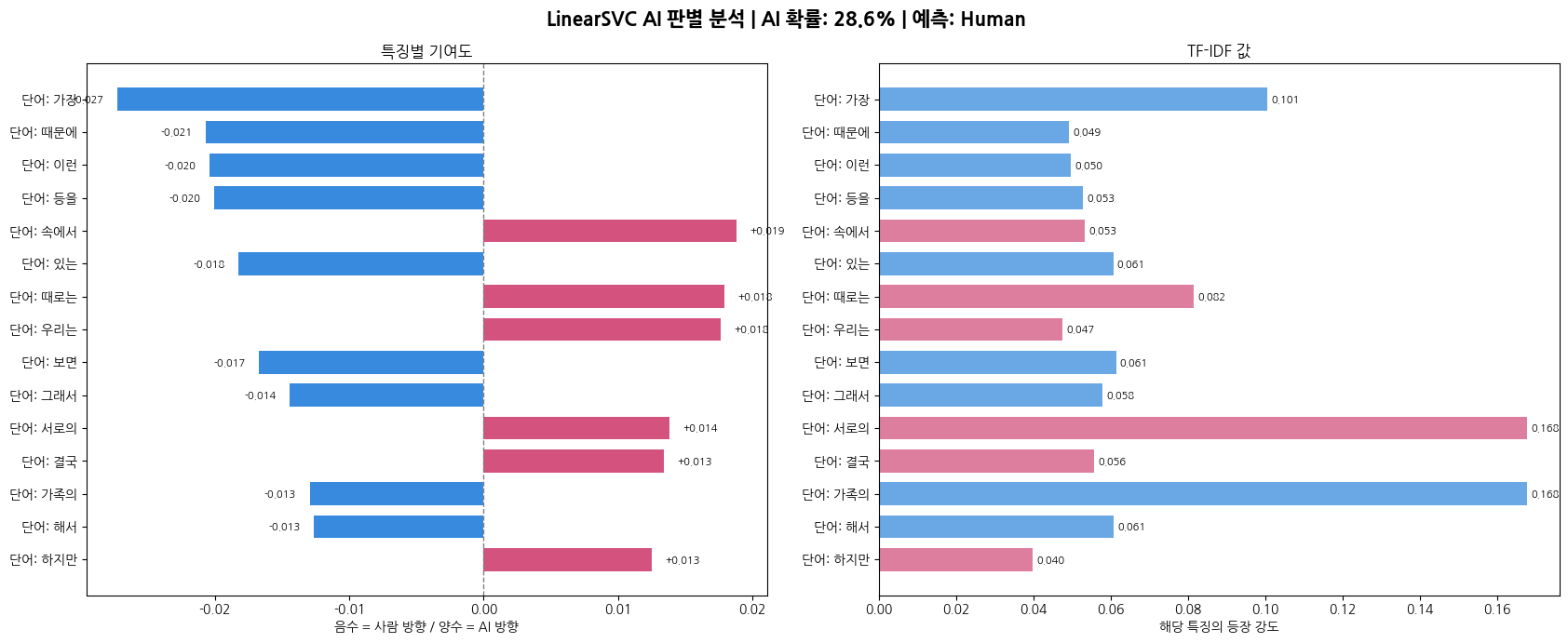
3-3. LinearSVC의 특징

Logistic Regression과 동일한 TF-IDF를 쓰지만 분류기를 Support Vector Machine으로 교체함. LinearSVC는 고차원 희소 벡텅에서 Logistic Regression보다 margin을 더 잘 최대화하는 경향이 있음.

3-4. 이 모델을 사용한 이유

TF-IDF 공간처럼 feature 수가 매우 많고 데이터가 희소한 텍스트 분류 문제에서 SVM은 강한 성능을 보임. 확률 출력이 필요하여 CalibratedClassifierCV로 감쌌음.

4. Voting Ensemble

4-1. 모델 코드 및 결과

모델 코드

import pickle
import pandas as pd

from sklearn.model_selection import train_test_split, cross_val_score, StratifiedKFold
from sklearn.pipeline import Pipeline, FeatureUnion
from sklearn.feature_extraction.text import TfidfVectorizer
from sklearn.linear_model import LogisticRegression
from sklearn.svm import LinearSVC
from sklearn.calibration import CalibratedClassifierCV
from sklearn.naive_bayes import ComplementNB
from sklearn.ensemble import VotingClassifier
from sklearn.metrics import accuracy_score, classification_report, confusion_matrix, f1_score


# ─────────────────────────────────────────
# 1. 데이터 로드
# ─────────────────────────────────────────
data = pd.read_csv("labeled_dataset.csv").dropna(subset=["text", "label"]).copy()
data["text"] = data["text"].astype(str)
data["label"] = data["label"].astype(int)

print(f"총 데이터: {len(data)}건")
print(f"Human: {(data['label'] == 0).sum()}건")
print(f"AI: {(data['label'] == 1).sum()}건")


# ─────────────────────────────────────────
# 2. 학습 / 테스트 분리
# ─────────────────────────────────────────
X_train, X_test, y_train, y_test = train_test_split(
    data["text"],
    data["label"],
    test_size=0.2,
    random_state=42,
    stratify=data["label"]
)


# ─────────────────────────────────────────
# 3. Feature 구성
# ─────────────────────────────────────────
features = FeatureUnion([
    ("char_tfidf", TfidfVectorizer(
        analyzer="char",
        ngram_range=(3, 5),
        min_df=2,
        max_features=50000,
        sublinear_tf=True,
        lowercase=False
    )),
    ("word_tfidf", TfidfVectorizer(
        analyzer="word",
        ngram_range=(1, 2),
        min_df=2,
        max_features=30000,
        sublinear_tf=True,
        lowercase=False
    ))
])


# ─────────────────────────────────────────
# 4. 개별 모델 구성
# ─────────────────────────────────────────
lr = LogisticRegression(
    solver="saga",
    max_iter=3000,
    C=2.0,
    class_weight="balanced",
    n_jobs=-1,
    random_state=42
)

svc = CalibratedClassifierCV(
    LinearSVC(
        C=1.0,
        class_weight="balanced",
        random_state=42,
        max_iter=5000
    ),
    cv=3
)

nb = ComplementNB(alpha=0.5)


# ─────────────────────────────────────────
# 5. Voting Ensemble 구성
# ─────────────────────────────────────────
ensemble_clf = VotingClassifier(
    estimators=[
        ("lr", lr),
        ("svc", svc),
        ("nb", nb)
    ],
    voting="soft"
)

model = Pipeline([
    ("features", features),
    ("clf", ensemble_clf)
])


# ─────────────────────────────────────────
# 6. 학습
# ─────────────────────────────────────────
print("\n[Voting Ensemble 학습 시작]")
model.fit(X_train, y_train)


# ─────────────────────────────────────────
# 7. 테스트 평가
# ─────────────────────────────────────────
y_pred = model.predict(X_test)

print("\n=== Voting Ensemble Test 성능 ===")
print(f"Accuracy: {accuracy_score(y_test, y_pred) * 100:.2f}%")
print(f"F1 macro: {f1_score(y_test, y_pred, average='macro'):.4f}")
print(classification_report(y_test, y_pred, target_names=["Human", "AI"], zero_division=0))
print("Confusion matrix:")
print(confusion_matrix(y_test, y_pred))


# ─────────────────────────────────────────
# 8. 교차검증
# ─────────────────────────────────────────
cv = StratifiedKFold(n_splits=3, shuffle=True, random_state=42)

cv_scores = cross_val_score(
    model,
    data["text"],
    data["label"],
    cv=cv,
    scoring="f1_macro",
    n_jobs=-1
)

print("\n=== 3-fold CV ===")
print(f"f1_macro: {cv_scores.mean():.4f} (± {cv_scores.std():.4f})")


# ─────────────────────────────────────────
# 9. 저장
# ─────────────────────────────────────────
with open("ai_detector_ensemble.pkl", "wb") as f:
    pickle.dump(model, f)

print("\n모델 저장 완료: ai_detector_ensemble.pkl")

결과

총 데이터: 2400건  
Human: 1200건  
AI: 1200건

\[Voting Ensemble 학습 시작\]

\=== Voting Ensemble Test 성능 ===  
Accuracy: 99.38%  
F1 macro: 0.9937  
precision recall f1-score support

```
   Human       1.00      0.99      0.99       240
      AI       0.99      1.00      0.99       240

accuracy                           0.99       480
```

macro avg 0.99 0.99 0.99 480  
weighted avg 0.99 0.99 0.99 480

Confusion matrix:  
\[\[237 3\]  
\[ 0 240\]\]

\=== 3-fold CV ===  
f1\_macro: 0.9837 (± 0.0027)

모델 저장 완료: ai\_detector\_ensemble.pkl

4-2. 실제 테스트 코드 및 결과

테스트 코드

import pickle
import numpy as np
import matplotlib.pyplot as plt

# 한글 폰트 깨지면 사용
# import koreanize_matplotlib


# ─────────────────────────────────────────
# 1. Voting Ensemble 모델 로드
# ─────────────────────────────────────────
MODEL_PATH = "ai_detector_ensemble.pkl"

with open(MODEL_PATH, "rb") as f:
    model = pickle.load(f)

print(f"모델 로드 완료: {MODEL_PATH}")


# ─────────────────────────────────────────
# 2. Pipeline 내부 구조 꺼내기
# ─────────────────────────────────────────
features = model.named_steps["features"]
voting_clf = model.named_steps["clf"]


# ─────────────────────────────────────────
# 3. FeatureUnion feature 이름 가져오기
# ─────────────────────────────────────────
def get_feature_names_from_union(feature_union):
    feature_names = []

    for name, transformer in feature_union.transformer_list:
        names = transformer.get_feature_names_out()
        names = [f"{name}__{feature}" for feature in names]
        feature_names.extend(names)

    return np.array(feature_names)


feature_names = get_feature_names_from_union(features)


# ─────────────────────────────────────────
# 4. Calibrated LinearSVC 계수 꺼내기
# ─────────────────────────────────────────
def get_coef_from_calibrated_svc(clf):
    """
    CalibratedClassifierCV 내부 LinearSVC들의 coef_를 평균내서 가져온다.
    """

    if hasattr(clf, "coef_"):
        return clf.coef_[0]

    if hasattr(clf, "calibrated_classifiers_"):
        coefs = []

        for calibrated_clf in clf.calibrated_classifiers_:
            base_estimator = getattr(calibrated_clf, "estimator", None)

            if base_estimator is None:
                base_estimator = getattr(calibrated_clf, "base_estimator", None)

            if base_estimator is not None and hasattr(base_estimator, "coef_"):
                coefs.append(base_estimator.coef_[0])

        if len(coefs) > 0:
            return np.mean(coefs, axis=0)

    raise AttributeError("LinearSVC 계수를 가져올 수 없습니다.")


# ─────────────────────────────────────────
# 5. 개별 모델별 AI 확률 가져오기
# ─────────────────────────────────────────
def get_individual_model_probs(X):
    """
    VotingClassifier 안에 들어간 개별 모델들의 AI 확률을 가져온다.
    """

    result = {}

    for name, estimator in voting_clf.named_estimators_.items():
        if hasattr(estimator, "predict_proba"):
            prob = estimator.predict_proba(X)[0][1]
            result[name] = prob

    return result


# ─────────────────────────────────────────
# 6. Ensemble feature 기여도 계산
# ─────────────────────────────────────────
def get_ensemble_contribution_vector():
    """
    Voting Ensemble 내부 모델들의 계수를 이용해 설명용 contribution vector를 만든다.

    사용 모델:
    - Logistic Regression: coef_
    - Calibrated LinearSVC: 내부 LinearSVC coef_ 평균
    - ComplementNB: feature_log_prob_ 차이

    주의:
    Voting Ensemble의 실제 판단은 세 모델의 확률 평균이므로,
    이 기여도는 '설명용 근사값'이다.
    """

    contribution_vectors = []

    for name, estimator in voting_clf.named_estimators_.items():

        # 1. Logistic Regression
        if hasattr(estimator, "coef_"):
            contribution_vectors.append(estimator.coef_[0])

        # 2. Calibrated LinearSVC
        elif hasattr(estimator, "calibrated_classifiers_"):
            try:
                svc_coef = get_coef_from_calibrated_svc(estimator)
                contribution_vectors.append(svc_coef)
            except AttributeError:
                pass

        # 3. Naive Bayes 계열
        elif hasattr(estimator, "feature_log_prob_"):
            # class 1(AI) 쪽 log prob - class 0(Human) 쪽 log prob
            nb_coef = estimator.feature_log_prob_[1] - estimator.feature_log_prob_[0]
            contribution_vectors.append(nb_coef)

    if len(contribution_vectors) == 0:
        raise AttributeError("Ensemble 내부에서 설명 가능한 계수를 찾지 못했습니다.")

    # 모델마다 계수 스케일이 다를 수 있어서 표준화 후 평균
    normalized_vectors = []

    for vec in contribution_vectors:
        std = np.std(vec)

        if std == 0:
            normalized_vectors.append(vec)
        else:
            normalized_vectors.append((vec - np.mean(vec)) / std)

    return np.mean(normalized_vectors, axis=0)


ensemble_coef = get_ensemble_contribution_vector()


# ─────────────────────────────────────────
# 7. 단순 판별 함수
# ─────────────────────────────────────────
def detect_ai(text: str):
    prob = model.predict_proba([text])[0][1]
    pred = model.predict([text])[0]

    print("\n" + "=" * 80)
    print("입력 텍스트:")
    print(text[:500] + "..." if len(text) > 500 else text)
    print("-" * 80)
    print(f"예측 라벨: {'AI' if pred == 1 else 'Human'}")
    print(f"AI 확률: {prob * 100:.2f}%")

    if prob >= 0.7:
        print("최종 해석: AI 작성 가능성이 높음")
    elif prob >= 0.4:
        print("최종 해석: 애매함")
    else:
        print("최종 해석: 사람이 작성했을 가능성이 높음")

    print("=" * 80)

    return prob


# ─────────────────────────────────────────
# 8. Voting Ensemble 설명 + 시각화 함수
# ─────────────────────────────────────────
def explain_ensemble(text, top_n=15, save_path="ensemble_explain_result.png"):
    # 텍스트 벡터화
    X = features.transform([text])

    # 최종 예측
    final_prob = model.predict_proba([text])[0][1]
    final_pred = model.predict([text])[0]

    # 개별 모델 확률
    individual_probs = get_individual_model_probs(X)

    # 현재 문서에 실제 등장한 feature
    indices = X.indices
    values = X.data

    # feature별 기여도
    contributions = values * ensemble_coef[indices]

    # 상위 feature 추출
    order = np.argsort(np.abs(contributions))[::-1][:top_n]

    top_features = feature_names[indices][order]
    top_contribs = contributions[order]
    top_values = values[order]

    display_features = [
        feat.replace("char_tfidf__", "문자: ")
            .replace("word_tfidf__", "단어: ")
        for feat in top_features
    ]

    # ─────────────────────────────────────
    # 텍스트 출력
    # ─────────────────────────────────────
    print("\n" + "=" * 90)
    print(f"입력 텍스트: {text[:100]}{'...' if len(text) > 100 else ''}")
    print(f"Voting Ensemble 예측 라벨: {'AI' if final_pred == 1 else 'Human'}")
    print(f"Voting Ensemble AI 확률: {final_prob * 100:.2f}%")
    print("=" * 90)

    print("\n[개별 모델별 AI 확률]")
    for name, prob in individual_probs.items():
        print(f"{name:<10}: {prob * 100:.2f}%")

    print(f"\n{'특징':<35} {'TF-IDF':>10} {'기여도':>12} 방향")
    print("-" * 90)

    for feat, val, contrib in zip(display_features, top_values, top_contribs):
        direction = "→ AI" if contrib > 0 else "→ 사람"
        print(f"{feat:<35} {val:>10.4f} {contrib:>+12.4f} {direction}")

    # ─────────────────────────────────────
    # matplotlib 시각화
    # ─────────────────────────────────────
    fig, axes = plt.subplots(1, 3, figsize=(23, 7))

    fig.suptitle(
        f"Voting Ensemble AI 판별 분석 | AI 확률: {final_prob * 100:.1f}% | 예측: {'AI' if final_pred == 1 else 'Human'}",
        fontsize=16,
        fontweight="bold"
    )

    # ── 그래프 1: 개별 모델별 AI 확률 ─────────
    ax0 = axes[0]

    model_names = list(individual_probs.keys())
    model_probs = [individual_probs[name] * 100 for name in model_names]

    bars0 = ax0.bar(model_names, model_probs)

    ax0.axhline(50, color="gray", linestyle="--", linewidth=1)
    ax0.set_ylim(0, 100)
    ax0.set_title("개별 모델별 AI 확률")
    ax0.set_ylabel("AI 확률 (%)")
    ax0.set_xlabel("모델")

    for bar, val in zip(bars0, model_probs):
        ax0.text(
            bar.get_x() + bar.get_width() / 2,
            val + 1,
            f"{val:.1f}%",
            ha="center",
            va="bottom",
            fontsize=9
        )

    # ── 그래프 2: 특징별 기여도 ─────────────
    y_pos = np.arange(len(display_features))

    reversed_features = display_features[::-1]
    reversed_contribs = top_contribs[::-1]
    reversed_values = top_values[::-1]

    colors = ["#D4537E" if c > 0 else "#378ADD" for c in reversed_contribs]

    ax1 = axes[1]

    bars1 = ax1.barh(
        y_pos,
        reversed_contribs,
        color=colors,
        height=0.7
    )

    ax1.set_yticks(y_pos)
    ax1.set_yticklabels(reversed_features)
    ax1.axvline(0, color="gray", linestyle="--", linewidth=1)
    ax1.set_title("특징별 기여도")
    ax1.set_xlabel("음수 = 사람 방향 / 양수 = AI 방향")

    for bar, val in zip(bars1, reversed_contribs):
        ax1.text(
            val + (0.001 if val >= 0 else -0.001),
            bar.get_y() + bar.get_height() / 2,
            f"{val:+.3f}",
            va="center",
            ha="left" if val >= 0 else "right",
            fontsize=8
        )

    # ── 그래프 3: TF-IDF 값 ─────────────────
    ax2 = axes[2]

    bars2 = ax2.barh(
        y_pos,
        reversed_values,
        color=colors,
        alpha=0.75,
        height=0.7
    )

    ax2.set_yticks(y_pos)
    ax2.set_yticklabels(reversed_features)
    ax2.set_title("TF-IDF 값")
    ax2.set_xlabel("해당 특징의 등장 강도")

    for bar, val in zip(bars2, reversed_values):
        ax2.text(
            val + 0.001,
            bar.get_y() + bar.get_height() / 2,
            f"{val:.3f}",
            va="center",
            ha="left",
            fontsize=8
        )

    plt.tight_layout()
    plt.savefig(save_path, dpi=150, bbox_inches="tight")
    plt.show()

    print(f"\n시각화 저장 완료: {save_path}")
    print("=" * 90 + "\n")

my_text = """
"""

ai_text = """

"""

explain_ensemble(human_text, save_path="ensemble_human_result.png")
explain_ensemble(ai_text, save_path="ensemble_ai_result.png")

결과

1. 사람이 쓴 글

\[개별 모델별 AI 확률\]  
lr : 24.71%  
svc : 2.05%  
nb : 8.34%

2. AI가 쓴 글

[개별 모델별 AI 확률]  
lr : 43.58%  
svc : 28.55%  
nb : 89.99%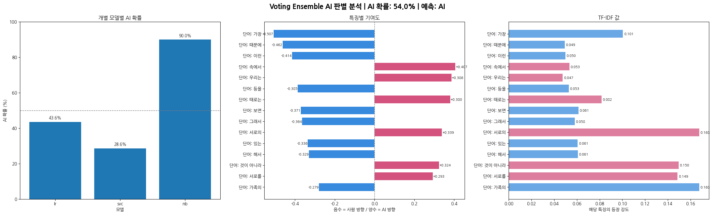

4-3. 앙상블 구성

세 개의 모델을 soft voting으로 결합함.

1. Logistic Regression: 선형, 확률 직접 출력
2. Linear SVC: 마진 기반, 고차원 텍스트에 강함
3. ComplementNB: 불균형 클래스에 강한 Naive Bayes 변형

4-4. 이 모델을 사용한 이유

단일 모델은 각자의 약점이 있는데, 여러 모델이 독립적으로 판단한 후 확률을 평균내면 한 모델이 틀려도 나머지가 보완이 가능함. 특히 ComplementNB는 어느 한 쪽 클래스 데이터가 적을 때도 잘 동작하여 다양성 측면에서 추가함.

5. BERT

5-1. 모델 코드 및 결과

모델 코드

import pandas as pd
import numpy as np
import torch

from torch.utils.data import Dataset

from sklearn.model_selection import train_test_split
from sklearn.metrics import (
    accuracy_score,
    precision_recall_fscore_support,
    confusion_matrix,
    classification_report
)

from transformers import (
    AutoTokenizer,
    AutoModelForSequenceClassification,
    TrainingArguments,
    Trainer
)


# ─────────────────────────────────────────
# 1. 기본 설정
# ─────────────────────────────────────────
MODEL_NAME = "klue/bert-base"
DATA_PATH = "labeled_dataset.csv"
SAVE_DIR = "./ai_detector_bert"

MAX_LENGTH = 256
RANDOM_STATE = 42


# ─────────────────────────────────────────
# 2. 데이터 로드
# ─────────────────────────────────────────
data = pd.read_csv(DATA_PATH).dropna(subset=["text", "label"]).copy()
data["text"] = data["text"].astype(str)
data["label"] = data["label"].astype(int)

print(f"총 데이터: {len(data)}건")
print(f"Human: {(data['label'] == 0).sum()}건")
print(f"AI: {(data['label'] == 1).sum()}건")


# ─────────────────────────────────────────
# 3. 학습 / 테스트 분리
# ─────────────────────────────────────────
train_df, test_df = train_test_split(
    data,
    test_size=0.2,
    random_state=RANDOM_STATE,
    stratify=data["label"]
)

print(f"Train: {len(train_df)}건")
print(f"Test: {len(test_df)}건")


# ─────────────────────────────────────────
# 4. Tokenizer 로드
# ─────────────────────────────────────────
tokenizer = AutoTokenizer.from_pretrained(MODEL_NAME)


# ─────────────────────────────────────────
# 5. PyTorch Dataset 직접 만들기
# ─────────────────────────────────────────
class TextClassificationDataset(Dataset):
    def __init__(self, texts, labels, tokenizer, max_length=256):
        self.texts = list(texts)
        self.labels = list(labels)
        self.tokenizer = tokenizer
        self.max_length = max_length

    def __len__(self):
        return len(self.texts)

    def __getitem__(self, idx):
        text = str(self.texts[idx])
        label = int(self.labels[idx])

        encoding = self.tokenizer(
            text,
            truncation=True,
            padding="max_length",
            max_length=self.max_length,
            return_tensors="pt"
        )

        item = {
            "input_ids": encoding["input_ids"].squeeze(0),
            "attention_mask": encoding["attention_mask"].squeeze(0),
            "labels": torch.tensor(label, dtype=torch.long)
        }

        if "token_type_ids" in encoding:
            item["token_type_ids"] = encoding["token_type_ids"].squeeze(0)

        return item


train_dataset = TextClassificationDataset(
    train_df["text"],
    train_df["label"],
    tokenizer,
    max_length=MAX_LENGTH
)

test_dataset = TextClassificationDataset(
    test_df["text"],
    test_df["label"],
    tokenizer,
    max_length=MAX_LENGTH
)


# ─────────────────────────────────────────
# 6. 모델 로드
# ─────────────────────────────────────────
model = AutoModelForSequenceClassification.from_pretrained(
    MODEL_NAME,
    num_labels=2
)


# ─────────────────────────────────────────
# 7. 평가 함수
# ─────────────────────────────────────────
def compute_metrics(eval_pred):
    logits, labels = eval_pred
    preds = np.argmax(logits, axis=1)

    precision, recall, f1, _ = precision_recall_fscore_support(
        labels,
        preds,
        average="macro",
        zero_division=0
    )

    acc = accuracy_score(labels, preds)

    return {
        "accuracy": acc,
        "f1_macro": f1,
        "precision_macro": precision,
        "recall_macro": recall
    }


# ─────────────────────────────────────────
# 8. 학습 설정
# ─────────────────────────────────────────
training_args = TrainingArguments(
    output_dir=SAVE_DIR,
    eval_strategy="epoch",
    save_strategy="epoch",

    learning_rate=2e-5,
    per_device_train_batch_size=8,
    per_device_eval_batch_size=8,
    num_train_epochs=3,
    weight_decay=0.01,

    logging_steps=20,

    load_best_model_at_end=True,
    metric_for_best_model="f1_macro",
    greater_is_better=True,

    save_total_limit=2,
    report_to="none"
)


# ─────────────────────────────────────────
# 9. Trainer 구성
# ─────────────────────────────────────────
trainer = Trainer(
    model=model,
    args=training_args,
    train_dataset=train_dataset,
    eval_dataset=test_dataset,
    compute_metrics=compute_metrics
)


# ─────────────────────────────────────────
# 10. 학습
# ─────────────────────────────────────────
print("\n[BERT 학습 시작]")
trainer.train()


# ─────────────────────────────────────────
# 11. 최종 평가
# ─────────────────────────────────────────
print("\n[BERT 평가 시작]")
pred_output = trainer.predict(test_dataset)

logits = pred_output.predictions
y_true = pred_output.label_ids
y_pred = np.argmax(logits, axis=1)

print("\n=== BERT Test 성능 ===")
print(f"Accuracy: {accuracy_score(y_true, y_pred) * 100:.2f}%")
print(classification_report(y_true, y_pred, target_names=["Human", "AI"], zero_division=0))
print("Confusion matrix:")
print(confusion_matrix(y_true, y_pred))


# ─────────────────────────────────────────
# 12. 모델 저장
# ─────────────────────────────────────────
trainer.save_model(SAVE_DIR)
tokenizer.save_pretrained(SAVE_DIR)

print(f"\nBERT 모델 저장 완료: {SAVE_DIR}")

결과

\[BERT 평가 시작\]

\=== BERT Test 성능 ===  
Accuracy: 99.58%  
precision recall f1-score support

Human 1.00 0.99 1.00 240
AI 0.99 1.00 1.00 240

accuracy 1.00 480

macro avg 1.00 1.00 1.00 480
weighted avg 1.00 1.00 1.00 480

Confusion matrix:
[[238 2]
[ 0 240]]
Writing model shards: 100%
 1/1 [00:01<00:00,  1.58s/it]

BERT 모델 저장 완료: ./ai_detector_bert

5-2. 실제 테스트 코드 및 결과

테스트 코드

import torch
import torch.nn.functional as F
import numpy as np
import matplotlib.pyplot as plt

from transformers import AutoTokenizer, AutoModelForSequenceClassification
import koreanize_matplotlib


# ─────────────────────────────────────────
# 1. BERT 모델 로드
# ─────────────────────────────────────────
MODEL_DIR = "./ai_detector_bert"

tokenizer = AutoTokenizer.from_pretrained(MODEL_DIR)
model = AutoModelForSequenceClassification.from_pretrained(MODEL_DIR)

device = torch.device("cuda" if torch.cuda.is_available() else "cpu")
model.to(device)
model.eval()

print(f"모델 로드 완료: {MODEL_DIR}")
print(f"사용 장치: {device}")


# ─────────────────────────────────────────
# 2. 토큰 정리 함수
# ─────────────────────────────────────────
def merge_subword_tokens(tokens, scores):
    """
    BERT WordPiece 토큰을 사람이 보기 좋게 합치는 함수.
    예: ['가', '##족'] → ['가족']

    scores는 subword 점수를 합산한다.
    """

    merged_tokens = []
    merged_scores = []

    special_tokens = {
        "[CLS]", "[SEP]", "[PAD]", "[UNK]",
        "<s>", "</s>", "<pad>"
    }

    for token, score in zip(tokens, scores):
        if token in special_tokens:
            continue

        # WordPiece 방식: ##로 시작하면 앞 토큰에 붙임
        if token.startswith("##"):
            if len(merged_tokens) > 0:
                merged_tokens[-1] += token[2:]
                merged_scores[-1] += score
            else:
                merged_tokens.append(token[2:])
                merged_scores.append(score)

        # SentencePiece 방식: ▁로 시작하면 새 단어 느낌
        elif token.startswith("▁"):
            merged_tokens.append(token.replace("▁", ""))
            merged_scores.append(score)

        else:
            merged_tokens.append(token)
            merged_scores.append(score)

    return merged_tokens, np.array(merged_scores)


# ─────────────────────────────────────────
# 3. 기본 판별 함수
# ─────────────────────────────────────────
def detect_ai_bert(text: str):
    inputs = tokenizer(
        text,
        return_tensors="pt",
        truncation=True,
        padding=True,
        max_length=256
    )

    inputs = {key: value.to(device) for key, value in inputs.items()}

    with torch.no_grad():
        outputs = model(**inputs)
        probs = F.softmax(outputs.logits, dim=1)[0]

    human_prob = probs[0].item()
    ai_prob = probs[1].item()
    pred = 1 if ai_prob >= human_prob else 0

    print("\n" + "=" * 80)
    print("입력 텍스트:")
    print(text[:500] + "..." if len(text) > 500 else text)
    print("-" * 80)
    print(f"Human 확률: {human_prob * 100:.2f}%")
    print(f"AI 확률: {ai_prob * 100:.2f}%")
    print(f"예측 라벨: {'AI' if pred == 1 else 'Human'}")

    if ai_prob >= 0.7:
        print("최종 해석: AI 작성 가능성이 높음")
    elif ai_prob >= 0.4:
        print("최종 해석: 애매함")
    else:
        print("최종 해석: 사람이 작성했을 가능성이 높음")

    print("=" * 80)

    return ai_prob


# ─────────────────────────────────────────
# 4. BERT 토큰 기여도 계산 함수
# ─────────────────────────────────────────
def get_token_contributions(text: str, max_length=256):
    """
    BERT의 입력 임베딩에 대한 gradient를 이용해서
    각 토큰이 AI class logit에 얼마나 영향을 주는지 계산한다.

    양수: AI 방향
    음수: Human 방향
    """

    model.zero_grad()

    encoded = tokenizer(
        text,
        return_tensors="pt",
        truncation=True,
        padding=True,
        max_length=max_length
    )

    input_ids = encoded["input_ids"].to(device)
    attention_mask = encoded["attention_mask"].to(device)

    token_type_ids = None
    if "token_type_ids" in encoded:
        token_type_ids = encoded["token_type_ids"].to(device)

    # input_ids를 직접 넣는 대신 embedding을 직접 만들어서 gradient를 추적
    embedding_layer = model.get_input_embeddings()
    embeds = embedding_layer(input_ids)
    embeds.retain_grad()

    forward_args = {
        "inputs_embeds": embeds,
        "attention_mask": attention_mask
    }

    if token_type_ids is not None:
        forward_args["token_type_ids"] = token_type_ids

    outputs = model(**forward_args)

    logits = outputs.logits
    probs = F.softmax(logits, dim=1)[0]

    human_prob = probs[0].item()
    ai_prob = probs[1].item()

    pred = torch.argmax(logits, dim=1).item()

    # AI class logit 기준으로 backward
    ai_logit = logits[0, 1]
    ai_logit.backward()

    grads = embeds.grad[0]
    embed_values = embeds.detach()[0]

    # signed contribution
    # 양수면 AI 방향, 음수면 Human 방향으로 해석
    token_scores = torch.sum(grads * embed_values, dim=1).detach().cpu().numpy()

    tokens = tokenizer.convert_ids_to_tokens(input_ids[0].detach().cpu().numpy())

    merged_tokens, merged_scores = merge_subword_tokens(tokens, token_scores)

    return {
        "tokens": merged_tokens,
        "scores": merged_scores,
        "human_prob": human_prob,
        "ai_prob": ai_prob,
        "pred": pred
    }


# ─────────────────────────────────────────
# 5. BERT 설명 + 시각화 함수
# ─────────────────────────────────────────
def explain_bert(text: str, top_n=15, save_path="bert_explain_result.png"):
    result = get_token_contributions(text)

    tokens = result["tokens"]
    scores = result["scores"]
    human_prob = result["human_prob"]
    ai_prob = result["ai_prob"]
    pred = result["pred"]

    if len(tokens) == 0:
        print("시각화할 토큰이 없습니다.")
        return

    # 절댓값 기준으로 영향이 큰 토큰 top_n개 선택
    order = np.argsort(np.abs(scores))[::-1][:top_n]

    top_tokens = np.array(tokens)[order]
    top_scores = scores[order]

    # 위에서부터 큰 값이 보이게 뒤집기
    reversed_tokens = top_tokens[::-1]
    reversed_scores = top_scores[::-1]

    # ─────────────────────────────────────
    # 텍스트 출력
    # ─────────────────────────────────────
    print("\n" + "=" * 90)
    print(f"입력 텍스트: {text[:100]}{'...' if len(text) > 100 else ''}")
    print(f"BERT 예측 라벨: {'AI' if pred == 1 else 'Human'}")
    print(f"Human 확률: {human_prob * 100:.2f}%")
    print(f"AI 확률: {ai_prob * 100:.2f}%")
    print("=" * 90)

    print(f"\n{'토큰':<20} {'기여도':>12} 방향")
    print("-" * 90)

    for token, score in zip(top_tokens, top_scores):
        direction = "→ AI" if score > 0 else "→ 사람"
        print(f"{token:<20} {score:>+12.4f} {direction}")

    # ─────────────────────────────────────
    # matplotlib 시각화
    # ─────────────────────────────────────
    fig, axes = plt.subplots(1, 2, figsize=(17, 7))

    fig.suptitle(
        f"BERT AI 판별 분석 | AI 확률: {ai_prob * 100:.1f}% | 예측: {'AI' if pred == 1 else 'Human'}",
        fontsize=15,
        fontweight="bold"
    )

    # ── 그래프 1: Human / AI 확률 ─────────────
    ax0 = axes[0]

    labels = ["Human", "AI"]
    probs = [human_prob * 100, ai_prob * 100]

    bars0 = ax0.bar(labels, probs)

    ax0.set_ylim(0, 100)
    ax0.axhline(50, color="gray", linestyle="--", linewidth=1)
    ax0.set_title("분류 확률")
    ax0.set_ylabel("확률 (%)")

    for bar, val in zip(bars0, probs):
        ax0.text(
            bar.get_x() + bar.get_width() / 2,
            val + 1,
            f"{val:.1f}%",
            ha="center",
            va="bottom",
            fontsize=10
        )

    # ── 그래프 2: 토큰별 기여도 ─────────────
    ax1 = axes[1]

    y_pos = np.arange(len(reversed_tokens))

    colors = ["#D4537E" if score > 0 else "#378ADD" for score in reversed_scores]

    bars1 = ax1.barh(
        y_pos,
        reversed_scores,
        color=colors,
        height=0.7
    )

    ax1.set_yticks(y_pos)
    ax1.set_yticklabels(reversed_tokens)
    ax1.axvline(0, color="gray", linestyle="--", linewidth=1)

    ax1.set_title("토큰별 기여도")
    ax1.set_xlabel("음수 = 사람 방향 / 양수 = AI 방향")

    for bar, val in zip(bars1, reversed_scores):
        ax1.text(
            val + (0.001 if val >= 0 else -0.001),
            bar.get_y() + bar.get_height() / 2,
            f"{val:+.3f}",
            va="center",
            ha="left" if val >= 0 else "right",
            fontsize=8
        )

    plt.tight_layout()
    plt.savefig(save_path, dpi=150, bbox_inches="tight")
    plt.show()

    print(f"\n시각화 저장 완료: {save_path}")
    print("=" * 90 + "\n")


# ─────────────────────────────────────────
# 6. 테스트 텍스트
# ─────────────────────────────────────────
human_text = """
가족을 주제로 한 작품을 보면 어김없이 생각나는 건 역시나 가족이다. 나는 가족은 애증이라고 몇 번이고 외쳐왔다. 가족을 사랑할 수 있지만, 가족에게서 받은 상처는 가족에 대한 감정을 사랑의 껍질을 한 증오로 바꾸었다. 그것이 옳다고 몇 번이고 믿어왔다. 내가 받은 상처는 사라지지 않을 거라고 확실하게 믿고 있었다.



그렇게나 증오했던 가족들이 떠오르는 건 어째서일까. 생전 처음으로 할아버지, 할머니께 용건 없이 전화를 드렸다. 죽을 만큼 밉다가도 가족에 관한 작품을 보면 제일 먼저 떠오르는 게 참 신기하다. 할아버지와는 20분이나 통화를 했다. 내가 공부가 재미있어졌다고 했더니 정말 뛸 듯이 좋아하시더라. 내가 돈 문제 말고 단순 안부 전화를 드렸더니 신나서 말이 많아지셨다. 그 모습을 화면 너머로 듣고 있자니 갑자기 눈물이 나왔다. 과거의 나에 대한 원망? 애증이었던 내 감정에 대한 혼란? 정확히 확언할 수 없었다.



할아버지는 내 어린 시절을 기억하고 계신다. 나조차 기억하지 못했던, 내 중학생 시절의 한 부분을. 내가 며칠을, 몇달을, 몇년을 미워했어도 할아버지는 그 자리에서 날 바라보고 계신다. 내가 미워했던 사람이 날 영원히 사랑하고 있다는 것을 온몸으로 깨닫는 순간, 눈물이 터져나왔다. 아마 할아버지도 알고 계시지 않았을까. 우는 걸 숨기기 위해 애써 노력했건만 눈물은 10분 내내 멈출 줄을 몰랐다.



애증이라, 이게 맞는 표현일까. 전화가 끝나고 계속해서 고민했다.



가족은 어쩌면 뒤늦게 추억하는 여름 같다. 한창일 때는 싫다가도, 뒤돌아서면 잊을 수 없는 내 추억의 한 부분.
"""

ai_text = """
가족은 우리가 가장 먼저 만나는 작은 사회이자, 삶이 힘들 때 다시 돌아갈 수 있는 마음의 집이다. 가족이라고 해서 늘 완벽하게 서로를 이해하는 것은 아니다. 때로는 사소한 말 한마디에 서운해지고, 서로의 생각이 달라 다투기도 한다. 하지만 시간이 지나고 보면 가족은 결국 나를 가장 오래 지켜봐 준 사람들이다. 내가 잘할 때만 곁에 있는 것이 아니라, 부족하고 흔들릴 때도 쉽게 등을 돌리지 않는 존재이기 때문이다.

가족의 소중함은 특별한 순간보다 평범한 일상 속에서 더 잘 드러난다. 아침에 건네는 짧은 인사, 밥은 먹었는지 묻는 말, 늦은 밤 돌아왔을 때 켜져 있는 불빛 같은 것들은 작지만 따뜻한 사랑의 표현이다. 우리는 이런 마음을 너무 익숙하게 받아들여 고마움을 잊을 때가 많다. 그러나 가족의 관심과 걱정은 당연한 것이 아니라, 서로를 아끼기 때문에 가능한 일이다.

가족은 혈연만으로 정해지는 것이 아니라 함께 시간을 보내고, 서로의 삶을 책임 있게 바라보는 관계라고 생각한다. 그래서 가족에게 필요한 것은 거창한 선물보다 이해하려는 태도와 고마움을 표현하는 말이다. 가까운 사이일수록 더 함부로 대하지 않고, 마음을 전하려는 노력이 필요하다. 가족은 내 삶의 출발점이자, 앞으로 나아갈 힘을 주는 가장 든든한 버팀목이다.

"""


# ─────────────────────────────────────────
# 7. 기본 테스트 실행
# ─────────────────────────────────────────
explain_bert(human_text, save_path="bert_human_result.png")
explain_bert(ai_text, save_path="bert_ai_result.png")

결과

1. 사람이 쓴 글

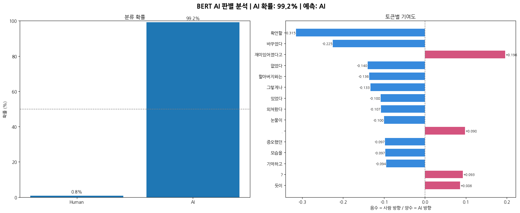
2. AI가 쓴 글

5-3. KLUE-BERT

앞의 모든 모델이 어떤 단어/글자 조합이 얼마나 자주 나오냐를 보는 것과 달리 문맥을 고려한 임베딩을 학습함. 같은 단어라도 앞뒤 문맥에 따라 다르게 표현된다는 점이 핵심적인 차이임. lue/bert-base를 파인튜닝해서 AI/Human 이진 분류에 적용함.

테스트 코드에서는 입력 임베딩에 대한 Gradient를 계산해서 각 토큰이 AI 판정에 얼마나 기여했는지를 시각화.

5-4. 이 모델을 사용한 이유

TF-IDF 기반 모델들은 단어의 위치나 문맥을 완전히 무시하는 bag of words 방식이라 미묘한 문체 차이를 잡기 어려움. BERT는 사전 학습된 언어 지식을 활용하여 훨씬 깊은 수준의 문체적 특징을 학습할 수 있고, 특히 한국어에 특화된 KLUE-BERT를 사용해서 한국어 텍스트 분류에 유리함.

5-5. 현재 BERT 적용 시 문제점

실제 사람이 쓴 글도 AI가 쓴 것 같다고 분류하고 있음. AI가 쓴 글과 확률이 크게 다르지 않은 점을 보아 모델 코드를 조금 더 손봐야 할 것으로 보임.

저작자표시 비영리 변경금지 (새창열림)

'인공지능 > 머신러닝' 카테고리의 다른 글

[팀 프로젝트] 심장병 분류 모델링 프로젝트 : Logistic Regression  (0)	2026.06.03